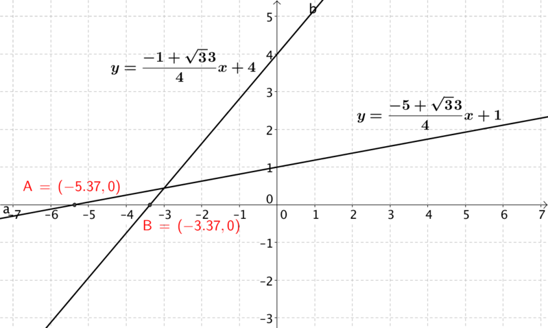
Straight line pairs

Straight line pairs

Excerpt: Can you find a pair of straight lines given a set of constraints linking their gradients and intercepts?

Problem

Construct a pair of straight lines whose $x$-intercepts differ by $2$, $y$-intercepts differ by $3$ and gradients differ by $1$.

Is there more than one way to do this?

You might find it helpful to try sketching your ideas on paper, or use graphing software such as Desmos.

Things you might have done

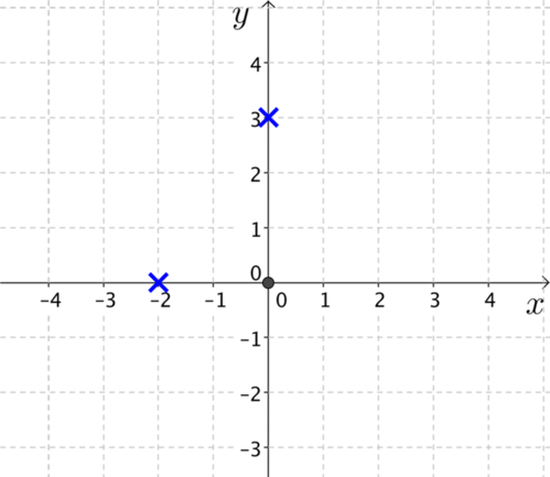
We might start by thinking about the specific case of a line going through the origin. We can then fix two points on a second line such that the $x$-intercepts differ by $2$ and the $y$-intercepts differ by $3$.

The final condition is that the gradients of the two lines differ by 1.

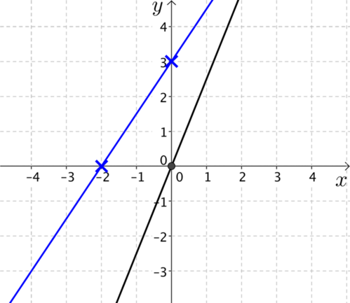
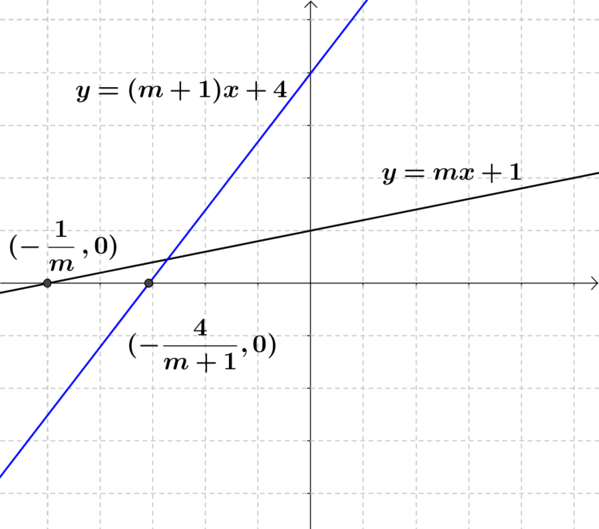
• What is the gradient of the blue line?

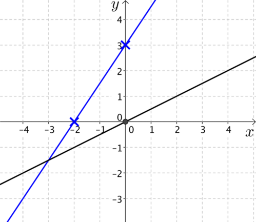
• Can you explain why the black line is a possible solution in each of the graphs below?

• What are the equations of each pair of lines?

This was a starting point that has successfully answered the question above, as we have already found two different solutions. We might now wonder …

• Are there any other pairs that you can create with a line through the origin as a starting point?

• How many pairs of lines are there in total?

Suggestion

Can you use this image to help you identify further solutions?

Trying to solve a problem by considering a specific case such as this, is often only the first step. The next step would be to try and generalise your findings. Some of the questions we could ask ourselves would be:

• Will this method work if the line doesn’t go through the origin?

We have found several pairs of lines that share a common feature, in this case, that one of the lines passes through the origin.

• Do you notice any symmetry appearing in your solutions?

• Do you think you will always be able to group pairs of lines together by a common $y$ intercept?

• What other common features could you use to group pairs together?

Once you have thought about this, have a look at the Taking it further section.

Taking it further

A possible first step to try to generalise our findings is to take a line that does not go through the origin.

Think about what was special about a line through the origin. Why did this make it a good starting point?

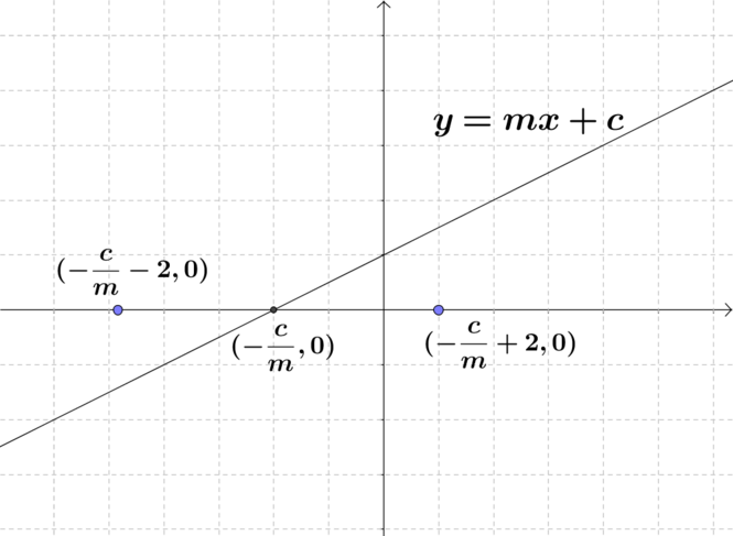
If we choose a line such as $y = x +1$ then we can draw points such that the $x$ intercepts differ by $2$ and the $y$ intercepts differ by $3$.

If we drew a line through these two points, would the two lines satisfy the required conditions?

By choosing $y = x +1$, we cannot modify the gradient or the intercepts of this line. Instead, perhaps it would be more useful to focus on one aspect. We could pick a point that the line passes through, or we could decide on the gradient of the line.

To explore a more general approach and get a feel for what is happening you can use the GeoGebra applet below or use this Desmos graph. You can click on the circles on the left to hide and show different lines as you wish.

Download GeoGebra file

Why are there four other lines along with the initial black line? Do these cover all possibilities? Could there be any other lines we should consider?

Below are discussions of three different approaches.

Fixing the gradient

It is perhaps easiest to visualise what the solutions will look like here compared to the two methods below. Given you know the gradients, the solutions will just be translations of the lines up and down the y axis.

Let’s start by picking a gradient of two and take our first line to be $y = 2x + c$. Then we can take the case where the second line has a gradient of $3$ and a $y$ intercept of $c + 3$.

When $y = 0$, the $x$ values will be $x= -\dfrac{c}{2}$ and $x = -\dfrac{c+3}{3}$.

The situation in the graph below is $-\dfrac{c}{2}-\left(-\dfrac{c+3}{3}\right) = 2$.

Subtracting the intercepts the other way $-\dfrac{c+3}{3}-\left(-\dfrac{c}{2}\right) = 2$ would come from a graph that looks like this.

What solutions arise from these two situations?

What sort of equations are you solving to find the solutions?

Can you find all the possible pairs of lines when the gradient is $2$? How many are there altogether?

If you take the lines to be $y = mx+c$ and $y = (m+1)x + c + 3$, can you find $c$ in terms of $m$? What sort of expression is it? You should end up with two solutions.

Can you continue to find all the possible solutions for $c$ in terms of $m$? You might start to notice some symmetry appearing…

Fixing the $y$ intercept

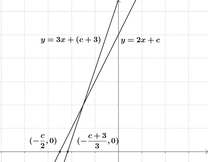
Let us take our first line to be $y= mx +1$. We can take the second line to be $y = (m+1)x + 4$.

Remember this is only one of four possibilities that the second line could be (think of the graph above).

We have our $y$ intercepts differing by three, we have our gradients differing by one, so we just need a difference of two in our $x$ intercepts.

When $y = 0$, $x = -\dfrac{1}{m}$ in our first line and $x = -\dfrac{4}{m+1}$ in our second.

We only want a ‘difference’ of $2$ in our $x$ intercepts, so we could subtract them either way round.

• Will both lead to solutions?

• How many solutions do you get?

If we continued with our line of $y = mx +1$ then what else could the second line be?

Remember we started with $y = (m+1)x + 4$. What can we change to find a different set of solutions?

Fixing the $x$ intercept

We are used to thinking about the $y$ intercept and the gradient when we deal with straight lines, so this may not have been an obvious place to start. However, this actually brings out the relationship between them quite nicely.

The $x$ intercept of this line is $x= -\dfrac{c}{m}$, so the $x$ intercept of the second line could be $x=-\dfrac{c}{m}-2$ or $x = -\dfrac{c}{m}+2$.

We have two possible $x$ intercepts and two possible gradients ($m+1$ and $m-1$). Choosing one of each should allow us to find the equation of a line.

You may find it beneficial to use the $y - y_0 = m(x - x_0)$ form of a straight line.

You should now have a line where the gradient differs by $1$ and the $x$ intercept by $2$ from the line $y = mx+c$.

Using the fact that the $y$ intercepts need to differ by three, can you form an equation in terms of $c$ and $m$?

Can you rearrange it to give you $c$ in terms of $m$?

Remember, we only chose one of our $x$ intercepts and one of our possible gradients. So are there more equations you could find linking $m$ and $c$? How many will there be altogether?

Taking it further solution

Below are the discussions of three approaches to finding a more general solution to the problem. They follow the Taking it further section but with more detailed solutions.

Fixing the gradient

This method keeps the calculations simple as it only involves solving linear equations.

Let’s start by picking a gradient of two and take our first line to be $y = 2x + c$. Then we can take the case where the second line has a gradient of $3$ and a $y$ intercept of $c + 3$.

When $y = 0$, the $x$ values will be $x= -\dfrac{c}{2}$ and $x = -\dfrac{c+3}{3}$.

The situation in the graph below is $-\dfrac{c}{2}-\left(-\dfrac{c+3}{3}\right) = 2$.

Subtracting the intercepts the other way $-\dfrac{c+3}{3}--\dfrac{c}{2} = 2$ would come from graphs that look like this.

Solving the equations leads to the solutions of $c= -6$ and $c = 18$. So two of the solutions when you start with $y = 2x + c$ are:

$$y = 2x - 6 \textrm { and } y = 3x - 3,$$

and

$$y = 2x + 18 \textrm { and } y = 3x + 21.$$

We chose the second line to be $y = (m+1)x + c+3$, which gave us two solutions. Putting the four different options together with the line $y = 2x+c$ would lead to $8$ pairs of solutions altogether.

Fixing the $y$ intercept

Let us take our first line to be $y= mx +1$. I will take the second line to be $y = (m+1)x + 4$. This is only one of four possibilities that the second line could be.

We have our $y$ intercepts differing by three, we have our gradient differing by one, so we just need the difference of two in our $x$ intercepts.

When $y = 0$, $x = -\dfrac{1}{m}$ in our first line and $x = -\dfrac{4}{m+1}$ in our second.

Starting with the following equation

$$-\dfrac{4}{m+1}-\left(-\dfrac{1}{m}\right)=2$$

leads to two solutions when you solve the quadratic $2m^2+5m-1=0$:

$$m = \dfrac{-5 \pm \sqrt{33}}{4}.$$

So there are two possible values for the gradient, giving us two different pairs of lines. One of these pairs is shown below.

Subtracting the intercepts the other way round leads to the quadratic $2m^2-m+1=0$ which has no real solutions. This is a nice link to a physical idea of what no solutions means here. Although it is possible to sketch the situation we were trying to solve (see the graph below), it will not be possible to find two lines that fit our constraints.

If you are not convinced, you might like to use the GeoGebra applet to try and find two lines that fit these constraints.

If you change the second line from $y = (m+1)x + 4$ to $y = (m+1)x - 2,$ $y = (m-1)x+4,$ $y = (m-1)x -2,$

then you can find the rest of the solutions for this case.

Fixing the $x$ intercept

This is not the obvious thing to start with, given our common form for the equation of a straight line which making it easier to think about ‘m’ and ‘c’. However, this actually brings out the relationship between them quite nicely.

The $x$ intercept of this line is $x= -\dfrac{c}{m}$ so the $x$ intercept of the second line could be $x=-\dfrac{c}{m}-2$ or $x = -\dfrac{c}{m}+2$.

This time instead of using $y = mx+c$ we can use the $y - y_0=m(x-x_0)$ form as we know the line is travelling through one of the points above.

If we take $(-\dfrac{c}{m}-2, 0)$, then $y_0=0$, $x_0=-\dfrac{c}{m}-2$ and we will take the gradient to be $m+1$. This gives us the equation:

$$y-0 = (m+1)(x - (-\frac{c}{m}-2)),$$

which simplifies to

$$y = (m+1)x + \frac{2m^2+2m+cm+c}{m}.$$

We want our $y$ intercepts to have a difference of $3$, so taking our two lines of

$$y = mx+c$$

and

$$y = (m+1)x + \frac{2m^2+2m+cm+c}{m},$$

we can subtract the intercepts to get

$$c - \frac{2m^2+2m+cm+c}{m}=3,$$

which we can rearrange to give us

$$c = -2m^2 - 5m.$$

If you subtracted the equations the other way around then you would get

$$c = m - 2m^2.$$

These are two of the possible expressions for c in terms of m.

There is a lot of scope to investigate this even further.

• You could find all the expressions for c in terms of m, and discuss the symmetry of them. (Graphing them would help).

• You may want to generalise beyond this example, and take the case where the difference between the $x$ intercepts is $p$, the $y$ intercepts is $q$ and the gradients is $r$.